Pima Indian 데이터를 이용한 결정 트리 분류

Pima Indians Diabetes Classification

sklearn 결정 트리를 이용한 분류

데이터 셋 출처

Pima Indians Diabetes Database | Kaggle
scikit-learn

사용 라이브러리

---

import numpy as np
import pandas as pd
import seaborn as sns
import matplotlib.pyplot as plt
import koreanize_matplotlib
from sklearn.model_selection import train_test_split
from sklearn.tree import plot_tree
from sklearn.metrics import accuracy_score

Data Load

df_pima = pd.read_csv("http://bit.ly/data-diabetes-csv")

---

EDA

df_pima.shape

(768, 9)

df_pima.sample(5)

	Pregnancies	Glucose	BloodPressure	SkinThickness	Insulin	BMI	DiabetesPedigreeFunction	Age	Outcome
141	5	106	82	30	0	39.5	0.286	38	0
370	3	173	82	48	465	38.4	2.137	25	1
712	10	129	62	36	0	41.2	0.441	38	1
49	7	105	0	0	0	0.0	0.305	24	0
605	1	124	60	32	0	35.8	0.514	21	0

df_pima.info()

<class 'pandas.core.frame.DataFrame'>
RangeIndex: 768 entries, 0 to 767
Data columns (total 9 columns):
 #   Column                    Non-Null Count  Dtype  
---  ------                    --------------  -----  
 0   Pregnancies               768 non-null    int64  
 1   Glucose                   768 non-null    int64  
 2   BloodPressure             768 non-null    int64  
 3   SkinThickness             768 non-null    int64  
 4   Insulin                   768 non-null    int64  
 5   BMI                       768 non-null    float64
 6   DiabetesPedigreeFunction  768 non-null    float64
 7   Age                       768 non-null    int64  
 8   Outcome                   768 non-null    int64  
dtypes: float64(2), int64(7)
memory usage: 54.1 KB

_ = df_pima.hist(figsize=(12, 8), bins=50)

9개의 열을 가진 768개의 데이터

df_pima.columns.tolist()

['Pregnancies',
 'Glucose',
 'BloodPressure',
 'SkinThickness',
 'Insulin',
 'BMI',
 'DiabetesPedigreeFunction',
 'Age',
 'Outcome']

• Pregnancies : 임신 횟수
• Glucose : 2시간 동안의 경구 포도당 내성 검사에서 혈장 포도당 농도
• BloodPressure : 이완기 혈압 (mm Hg)
• SkinThickness : 삼두근 피부 주름 두께 (mm) -> 체지방 추정용
• Insulin : 2시간 혈청 인슐린 (mu U / ml)
• BMI : 체질량 지수 (체중kg / 키(m)^2)
• DiabetesPedigreeFunction : 당뇨병 혈통 기능
• Age : 나이
• Outcome : 768개 중에 268개의 결과 클래스 변수(0 또는 1)는 1이고 나머지는 0

---

기본적인 학습

히스토그램을 보면, SkinThickness와 Insulin, BMI에 이상치가 있다는 사실을 확인 할 수 있지만,
일단 전처리를 하지 않은 상태에서 모델 성능 평가를해보고, 이후 하이퍼파라미터 튜닝을 진행하며 차이를 살펴 볼 예정

지도 학습의 경우 기본적으로 문제의 답을 알려줘야하는데, 해당 데이터 셋에서는 Outcome이 답에 해당함

---

Note!

하이퍼파라미터와 파라미터는 다름

• Hyperparameter (하이퍼파라미터)
  • 모델 학습 과정에 반영되는 값으로, 학습 전에 조절해야 됨
  • 학습률, 손실함수, 배치 사이즈 등
• Parameter (파라미터)
  • 모델 내부에서 결정되는 변수, 학습 또는 예측에 사용되는 값
  • 직접 조절이 불가능 함
  • 평균, 표준편차, 회귀 계수 가중치, 편향 등

하이퍼파라미터의 튜닝 방법은 굉장히 많음

---

데이터 셋 나누기

label_feature = "Outcome"
feature_name = df_pima.columns.tolist()
feature_name.remove(label_feature)

# train : test = 8 : 2로 나눔
split_count = int(df_pima.shape[0]*0.8)
train, test = df_pima[:split_count], df_pima[split_count:]
print(f"train: {train.shape}\ntest: {test.shape}")

train: (614, 9)
test: (154, 9)

X_train, y_train, X_test, y_test = train[feature_name], train[label_feature], test[feature_name], test[label_feature]
print(f"X_train: {X_train.shape}\y_train: {y_test.shape}\nX_test: {X_test.shape}\ny_test: {y_test.shape}")

X_train: (614, 8)
y_train: (614,)
X_test: (154, 8)
y_test: (154,)

# sklearn에서 제공하는 함수를 사용하면 훨씬 간편함
X_train, X_test, y_train, y_test = train_test_split(df_pima[feature_name], df_pima[label_feature], test_size=0.2, shuffle=False, random_state=42)
print(f"X_train: {X_train.shape}\ny_train: {y_train.shape}\nX_test: {X_test.shape}\ny_test: {y_test.shape}")

X_train: (614, 8)
y_train: (614,)
X_test: (154, 8)
y_test: (154,)

train_test_split은 sklearn 내장 메서드로 위 과정을 상단 부분 생략 가능함.
기본적인 파라미터는,

• arrays: 분할시킬 데이터
• test_size: 테스트 셋의 비율, default=0.25
• train_size: 학습 데이터 셋의 비율, defalut=1-test_size
• random_state
• shuffle: 기존 데이터를 나누기 전에 순서를 섞을것인지, default=True
• stratify: 지정한 데이터의 비율을 유지, 분류 문제의 경우 해당 옵션이 성능에 영향이 있다고는 함

---

머신러닝 알고리즘 사용

결정 트리 학습법 (Decision Tree Learning)

• 분류와 회귀에 모두 사용 가능한 CART (Classificaton and Regression Trees) 알고리즘
• 어떤 항목에 대한 관측값과 목표값을 연결 시켜주는 예측 모델로서 사용
  • 분류 트리: 목표 변수가 유한한 수의 값
  • 회귀 트리: 목표 변수가 연속하는 값
• 트리 최상단에는 가장 중요한 질문이 옴
• 결과를 해석(화이트박스 모델)하고 이해하기 쉬움
• 수치 / 범주형 자료에 모두 적용 가능
• 지니 불순도를 이용

결정 트리 학습법 종류

• 랜덤 포레스트
• 부스트 트리
• 회전 포레스트

지니 불순도 (Gini Impurity)

집합에 이질적인 것이 얼마나 섞여는지를 측정하는 지표
$I_G(f) = \sum_{i=1}^{m} f_i(1-f_i)$

• 불확실성을 의미 -> 얼마나 많은 것들이 섞여있는가?
• 한가지 특성을 가진 객체만 있을수록 집단을 설명하기 좋음
  • 특성이 동일해질수록 낮아짐
  • 특성이 다양할수록 높아짐

DecisionTreeClassifier(
    *,
    criterion='gini', # 분할방법 {"gini", "entropy"}, default="gini"
    splitter='best',
    max_depth=None, # The maximum depth of the tree
    min_samples_split=2, # The minimum number of samples required to split an internal node
    min_samples_leaf=1, # The minimum number of samples required to be at a leaf node.
    min_weight_fraction_leaf=0.0, # The minimum weighted fraction of the sum total of weights
    max_features=None, # 최적의 분할을 위해 고려하는 특성의 개수 (int -> 개수 / float -> 비율)
    random_state=None,
    max_leaf_nodes=None,
    min_impurity_decrease=0.0,
    class_weight=None,
    ccp_alpha=0.0,
)

• 주요 파라미터
  • criterion: 가지의 분할의 품질을 측정하는 방식
  • max_depth: 트리의 최대 깊이
  • min_samples_split:내부 노드를 분할하는 데 필요한 최소 샘플 수
  • min_samples_leaf: 리프 노드에 있어야 하는 최소 샘플 수
  • max_leaf_nodes: 리프 노드 숫자의 제한치
  • random_state: 추정기의 무작위성을 제어

from sklearn.tree import DecisionTreeClassifier
model = DecisionTreeClassifier(random_state=42)

# Train
model.fit(X_train, y_train)

DecisionTreeClassifier(random_state=42)

# Test
y_pre_1 = model.predict(X_test)

---

트리 알고리즘 분석

plt.figure(figsize=(24, 16))
plot_tree(model, filled=True, feature_names=feature_name)
plt.show()

지니 계수가 0이되면 트리 생성을 제한하는데, 파라미터 튜닝을 진행하지 않은 상황에서는 16개의 Leaf node가 존재함
그래프가 크므로 상위 4개 노드만 그려보면,

plt.figure(figsize=(12, 8))
plot_tree(model, filled=True, feature_names=feature_name, fontsize=8, max_depth=4)
plt.show()

결정 트리의 최상위에 Glucose가 온 것을 확인 할 수 있음
결정 트리의 최상단에는 가장 중요한 feature가 옴

---

특성(feature)의 중요도 추출하기

model.feature_importances_

array([0.05944171, 0.30368248, 0.13140431, 0.04020035, 0.09010707,
       0.15739296, 0.12077948, 0.09699165])

np.sum(model.feature_importances_)

1.0

_ = sns.barplot(x=model.feature_importances_, y=feature_name).set_title("Feature의 중요도")

---

성능 평가

성능 평가 방식은 다양하나 정확도만을 이용해 성능을 평가함

(y_test==y_pre_1).mean()

0.7142857142857143

위와 같은 방식으로 정확도를 구할 수 있지만, sklearn의 내장 함수를 사용

accuracy_score(y_test, y_pre_1)

0.7142857142857143

model.score(X_test, y_test)

0.7142857142857143

---

결정 트리 모델의 하이퍼파라미터 조절

모델을 생성 할 때, 기본적으로 주어지는 피처의 개수나 최대 높이를 제한해 모델을 생성하고 성능을 평가해봄

# 결정 트리 모델의 최대 높이를 4로 제한하고, 고려하는 특성의 비율도 0.8로 조절해서 모델을 생성
model = DecisionTreeClassifier(max_depth=4, max_features=0.8, random_state=42)
model.fit(X_train, y_train)
y_pre_max4 = model.predict(X_test)

accuracy_score(y_test, y_pre_max4)

0.7402597402597403

3점 정도의 성능 향상이 있음
모든 특성을 사용한다고 좋은 성능이 나오는 것은 아님

---

Feature Engineering

Garbage In - Garbage Out, 잘 전처리된 데이터를 사용하면 좋은 성능이 나온다는 의미
실제로 모델을 생성하기 이전에 EDA를 통해, 데이터를 분석하고 전처리하는 과정이 중요함

---

수치형 변수를 범주형 변수로 만들기

_ = df_pima["Pregnancies"].hist(bins=50).set_title("임신 횟수")

_ = sns.countplot(data=df_pima, x="Pregnancies", hue="Outcome")

Pima 인디언 데이터 셋에서 Pregnancies의 경우 3회 미만인 경우가 대부분임
0 ~ 17까지 수치형 범주지만, 범주형 변주로 바꾸는 피쳐 엔지니어링을 진행함 -> 임신 횟수 6회를 기준으로 범주형으로 전환

df_pima["Pregnancies_high"] = df_pima["Pregnancies"] > 6
df_pima.head(5)

	Pregnancies	Glucose	BloodPressure	SkinThickness	Insulin	BMI	DiabetesPedigreeFunction	Age	Outcome	Pregnancies_high
0	6	148	72	35	0	33.6	0.627	50	1	False
1	1	85	66	29	0	26.6	0.351	31	0	False
2	8	183	64	0	0	23.3	0.672	32	1	True
3	1	89	66	23	94	28.1	0.167	21	0	False
4	0	137	40	35	168	43.1	2.288	33	1	False

feature_name.remove("Pregnancies")
feature_name.append("Pregnancies_high")
feature_name

['Glucose',
 'BloodPressure',
 'SkinThickness',
 'Insulin',
 'BMI',
 'DiabetesPedigreeFunction',
 'Age',
 'Pregnancies_high']

X_train, X_test, y_train, y_test = train_test_split(df_pima[feature_name], df_pima[label_feature], test_size=0.2, shuffle=False, random_state=42)
model = DecisionTreeClassifier(max_depth=4, max_features=0.8, random_state=42)
model.fit(X_train, y_train)
y_pre_max4_Pre_high = model.predict(X_test)

accuracy_score(y_test, y_pre_max4_Pre_high)

0.7727272727272727

같은 모델에서, 하나의 특성만 수치형에서 범주형으로 변경했는데 3점 정도의 성능 향상이 있었음

---

결측치 처리하기

_ = df_pima["Insulin"].hist(bins=50).set_title("인슐린")

Insulin 항목의 경우 0으로 기입된 결측치가 많이 존재함

_ = sns.histplot(data=df_pima, x="Insulin", hue="Outcome", kde=True)

seaborn hist에서 kde(밀도 추정)을하면 해당 레이블의 밀도를 확인 가능함

df_pima["Insulin_nan"] = df_pima["Insulin"].replace(0, np.nan)
_ = sns.histplot(data=df_pima, x="Insulin_nan", hue="Outcome", kde=True)

df_pima["Insulin_nan"].isnull().mean()

0.4869791666666667

Insulin 항목에서 약 48%의 결측치가 존재함
결측치를 해결하는 방법은 여러가지가 존재하지만, 중앙값으로 대체하는 방식과 평균값으로 보완 두 가지 방식으로 진행

in_desc = df_pima.groupby("Outcome")["Insulin"].describe()
in_desc

	count	mean	std	min	25%	50%	75%	max
Outcome
0	500.0	68.792000	98.865289	0.0	0.0	39.0	105.00	744.0
1	268.0	100.335821	138.689125	0.0	0.0	0.0	167.25	846.0

feature_name.remove("Insulin")
feature_name.append("Insulin_filled")

---

중앙값 사용

df_pima["Insulin_filled"] = df_pima["Insulin_nan"]
df_pima.loc[(df_pima["Insulin_nan"].isnull()) & (df_pima["Outcome"]==1), "Insulin_filled"] = in_desc.loc[1, "50%"]
df_pima.loc[(df_pima["Insulin_nan"].isnull()) & (df_pima["Outcome"]==0), "Insulin_filled"] = in_desc.loc[0, "50%"]
df_pima["Insulin_filled"].isnull().sum()

0

X_train, X_test, y_train, y_test = train_test_split(df_pima[feature_name], df_pima[label_feature], test_size=0.2, shuffle=False, random_state=42)
model = DecisionTreeClassifier(max_depth=4, max_features=0.8, random_state=42)
model.fit(X_train, y_train)
y_pre_max4_50_per = model.predict(X_test)

accuracy_score(y_test, y_pre_max4_50_per)

0.8896103896103896

중앙값으로 Insulin의 결측치를 대체한 경우 약 11점 정도의 성능 향상이 있음

---

평균값 사용

df_pima["Insulin_filled"] = df_pima["Insulin_nan"]
df_pima.loc[(df_pima["Insulin_nan"].isnull()) & (df_pima["Outcome"]==1), "Insulin_filled"] = in_desc.loc[1, "mean"]
df_pima.loc[(df_pima["Insulin_nan"].isnull()) & (df_pima["Outcome"]==0), "Insulin_filled"] = in_desc.loc[0, "mean"]
df_pima["Insulin_filled"].isnull().sum()

0

X_train, X_test, y_train, y_test = train_test_split(df_pima[feature_name], df_pima[label_feature], test_size=0.2, shuffle=False, random_state=42)
model = DecisionTreeClassifier(max_depth=4, max_features=0.8, random_state=42)
model.fit(X_train, y_train)
y_pre_max4_mean = model.predict(X_test)

accuracy_score(y_test, y_pre_max4_mean)

0.8506493506493507

Insulin의 결측치를 처리하기 이전보다는 약 8점 정도의 성능 향상이 있지만, 중앙값으로 대체한 경우보다는 성능이 3점 정도 낮음

---

이상치(Outlier)

결측치 처리를 2가지 방식으로 했지만, 이상치를 분석하는 과정은 평균으로 처리한 경우를 다룸

plt.figure(figsize=(15, 2))
_ = sns.boxplot(x=df_pima["Insulin_filled"]).set_title("결측치를 평균으로 처리한 경우")

df_pima["Insulin_filled"].describe()

count    768.000000
mean     118.967780
std       93.557899
min       14.000000
25%       68.792000
50%      100.000000
75%      127.250000
max      846.000000
Name: Insulin_filled, dtype: float64

_ = sns.kdeplot(df_pima["Insulin_filled"]).set_title("이상치 처리 전")

결측치 문제를 해결했지만 이상치의 문제가 있음
75%가 넘어가는 부분을 평균으로 대체해줌

df_pima.loc[(df_pima["Insulin_filled"]>127.25) & (df_pima["Outcome"]==1), "Insulin_filled"] = in_desc.loc[1, "mean"]
df_pima.loc[(df_pima["Insulin_filled"]>127.25) & (df_pima["Outcome"]==0), "Insulin_filled"] = in_desc.loc[1, "mean"]

plt.figure(figsize=(15, 2))
_ = sns.boxplot(x=df_pima["Insulin_filled"]).set_title("이상치 처리 후")

_ = sns.kdeplot(df_pima["Insulin_filled"]).set_title("이상치 처리 후")

X_train, X_test, y_train, y_test = train_test_split(df_pima[feature_name], df_pima[label_feature], test_size=0.2, shuffle=False, random_state=42)
model = DecisionTreeClassifier(max_depth=4, max_features=0.8, random_state=42)
model.fit(X_train, y_train)
y_pre_max4_mean_out = model.predict(X_test)

accuracy_score(y_test, y_pre_max4_mean_out)

0.8441558441558441

이상치를 처리한 후에 성능이 조금 떨어졌음
통계를 기반으로하는 이상치 처리는 위험할 수도 있음
효과적인 이상치 탐색을 위해서는 해당 데이터 변수들의 의미와 도메인을 이해하고 원인을 파악하고 처리해야 됨

---

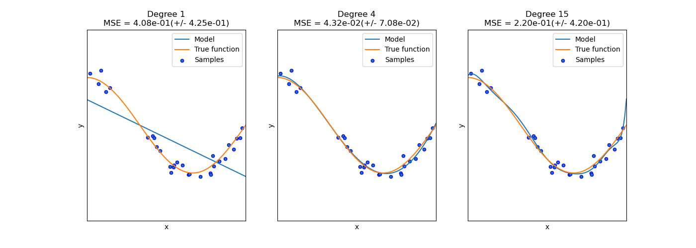
Overfitting과 Underfitting

해당 개념도 다뤄보고 싶은데, 사용한 데이터 셋의 크기가 작은 편이라 마땅한 방식을 생각하지 못해 개념만 소개하고 넘어가는걸로..

Overfitting (과적합)

Train 데이터에 과하게 영향을 받아, 훈련 평가 성능은 좋으나 테스트 평가 성능이 낮은 경우

Underfitting (과소적합)

Train 데이터의 양이 적어 학습을 제대로하지 못한 경우

이미지 출처: scikit learn